Core Syntax and Operations

Julia is fundamentally an imperative programming language, where the flow of execution is defined by sequences of commands or statements that change the program’s state. Core features include:

Assignment statements to store values in variables.
Control flows for decision-making and iteration.
Arithmetic operations for calculations.

While imperative programming emphasizes how a task is accomplished (e.g., through loops, conditionals, and assignments), declarative programming focuses on what the result should be, leaving the “how” to the language or framework. Julia is versatile and can incorporate elements of declarative programming, such as high-level operations on collections and functional programming paradigms, but its foundation is firmly rooted in imperative concepts.

Tip

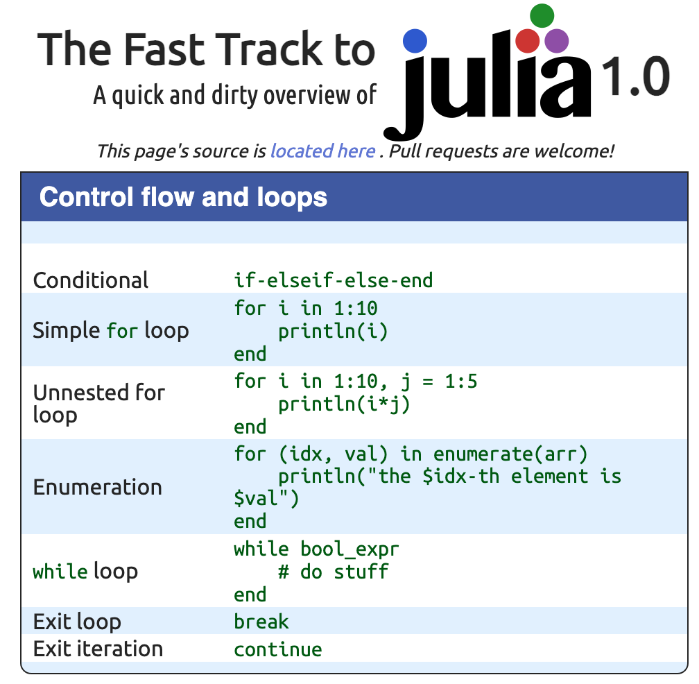
In this page, we present the fundamentals of Julia syntax. If you want a cheatsheet, click on the image below.

Basics

Assignment

In Julia, variables are assigned using the = operator:

x = 5
y = "Hello, Julia!"

Julia is dynamically typed, which means variables do not require explicit type declarations. Types are inferred based on the assigned value.

From math lectures, we recall 5 \in \mathbb{N}. We expect the outcome of the typeof function to tell us that x holds an integer.

typeof(x)

Int64

Indeed, Int64 is a label which refers to an integer storage format.

Similarly, the quotation marks around the sequence of characters show that y holds text, known as a string in programming languages—a way to represent words, sentences, or any combination of characters.

typeof(y)

String

The return value thus validates that the kind of data contained in y is a string. We would use the term character (Char in short) if y would hold a single basic unit of information (a letter, number, symbol, or control code), like in y = "a". Note that it is possible to indicate to Julia the kind of data we want a variable to hold, this is called annotating. For y to hold only sequences of characters, we would write y::String = "Hello, Julia!".

Variables act as labels pointing to values and can be reassigned without restrictions on type. This dynamic behavior is a hallmark of imperative languages.

Unicode Characters

Julia supports Unicode characters, enhancing code readability, especially for mathematical and scientific computations:

α = 10
β = α + 5
println("β = $β")

β = 15

Unicode symbols can be entered using \name followed by Tab (e.g., \alpha → α). A complete list of Unicode characters is available in the Julia Unicode documentation.

Comments

Comments are written with the # symbol. Julia also supports multiline comments with #= and =#:

# This is a single-line comment

#= 
This is a 
multiline comment 
=#

Printing Output

For debugging or displaying results, Julia provides the println function:

println("Hello, Julia!")  # Prints: Hello, Julia!
println("The value of α is ", α)

Hello, Julia!
The value of α is 10

Additionally, the @show macro prints both variable names and values:

x = 42
@show x   # Prints: x = 42

x = 42

You can also use @show with multiple variables or expressions:

a = 10
b = 20
@show a + b  # Prints: a + b = 30
@show a, b   # Prints: a = 10, b = 20

a + b = 30
(a, b) = (10, 20)

Comparison Operations

Julia includes standard comparison operators for equality and order:

Operator	Purpose	Example	Result
`==`	Equality check	`5 == 5`	`true`
`!=` or `≠`	Inequality check	`5 != 3`	`true`
`<`, `<=`	Less than, or equal	`5 < 10`	`true`
`===`	Object (type and value) identity check	`5 === 5.0`	`false`

Examples:

5 == 5     # true
5 != 3     # true
5 ≠ 3      # true (using Unicode)
5 < 10     # true
10 >= 10   # true
"Julia" === "Julia"  # true (identical strings)
5 === 5.0  # false (different types: Int vs. Float)

julia> 5 == 5 = true
julia> 5 != 3 = true
julia> 5 ≠ 3 = true
julia> 5 < 10 = true
julia> 10 >= 10 = true
julia> "Julia" === "Julia" = true
julia> 5 === 5.0 = false

Julia’s comparison operators return Bool values (true or false). Using these operators effectively is essential for control flow and logical expressions.

In Julia, the === operator checks object identity, meaning it determines if two references point to the exact same memory location or the same instance. This is a stricter comparison than ==, which only checks if two values are equivalent in terms of their contents, not if they are the same instance.

Here’s a breakdown of === in Julia:

Singletons: === is often used for checking singleton objects like nothing, true, false, and other immutable types that Julia reuses rather than copying. For instance, nothing === nothing will return true, and similarly, true === true will return true.
Immutable Types: For immutable types like Int, Float64, etc., === and == usually give the same result since identical values are often the same instance.
Performance: === is generally faster than == because it doesn’t need to do a value comparison, just a memory location check. This is particularly useful when checking if a value is a specific singleton (e.g., x === nothing).

a = 1
b = 1
a === b  # true, since 1 is an immutable integer, they are identical instances

x = [1, 2]
y = x
x === y  # true, because x and y refer to the same object in memory

x == [1, 2]   # true, because the contents are the same
x === [1, 2]  # false, because they are different instances in memory

julia> a = 1
julia> b = 1
julia> a === b = true
julia> x = [1, 2]
julia> y = [1, 2]
julia> x === y = true
julia> x == [1, 2] = true
julia> x === [1, 2] = false

In summary, === is especially useful for checking identity rather than equality, often applied to singletons or cases where knowing the exact instance matters, as it allows for efficient and clear comparisons.

Arithmetics

Julia supports a variety of arithmetic operations that can be performed on numeric types. Below are some of the most commonly used operations:

Basic Arithmetic Operations

You can perform basic arithmetic operations using standard operators:

Addition: +
Subtraction: -
Multiplication: *
Division: // (returns a rational number, the set \mathbb{Q}), / (returns a floating-point result, the set \mathbb{R} in finite precision)

a = 10
b = 3

sum = a + b
difference = a - b
product = a * b
quotient = a / b
rational = a // b

julia> a = 10
julia> b = 3
julia> sum = 13
julia> difference = 7
julia> product = 30
julia> quotient = 3.3333333333333335
julia> rational = 10//3

A number in \mathbb{Q} is written as a fraction of numbers from \mathbb{N}, designated with the label Int, short for integer. Numbers in \mathbb{R} can have infinite digits after the coma. These are truncated to be stored on a computer and designated by the label Float, short for floating-point number.

Modulo Operation

The modulo operator % returns the remainder of a division operation. It is useful for determining if a number is even or odd, or for wrapping around values.

modulus_result = a % b  # remainder of 10 divided by 3

Exponentiation

You can perform exponentiation using the ^ operator.

a^2          # 10 squared

Summary of Arithmetic Operations

Operation	Symbol	Example	Result
Addition	`+`	`5 + 3`	`8`
Subtraction	`-`	`5 - 3`	`2`
Multiplication	`*`	`5 * 3`	`15`
Division	`/`	`5 / 2`	`2.5`
Modulo	`%`	`5 % 2`	`1`
Exponentiation	`^`	`2 ^ 3`	`8`

These arithmetic operations can be combined and nested to perform complex calculations as needed.

Logical Operators

Julia includes standard logical operators, that combine or negate conditions:

Operator	Purpose	Example	Result
`&&`	Logical AND	`true && false`	`false`
`\|\|`	Logical OR	`true \|\| false`	`true`
`!`	Logical NOT	`!true`	`false`

a = true
b = false

a && b
a || b
!a

julia> a = true
julia> b = false
julia> a && b = false
julia> a || b = true
julia> !a = false

Data resulting from a computation with a logical operator can have only two possible values: true or false. This kind of data is refered to as a boolean, Bool in short.

Control Flows

Control flow in Julia is managed through conditional statements and loops. Logical operators allow for conditions to be combined or negated.

Conditional Statements

Julia supports if, elseif, and else for conditional checks:

x = 10

if x > 5
    println("x is greater than 5")
elseif x == 5
    println("x is equal to 5")
else
    println("x is less than 5")
end

x is greater than 5

In Julia, blocks for if, elseif, and else are closed with end. Indentation is not required by syntax but is recommended for readability.

Tip

You can follow the Blue Style conventions for Julia code. If you want to format your code you can use the package JuliaFormatter.jl.

Using Arithmetic in Control Flow

You can combine arithmetic operations with control flow statements. For example, you can use the modulo operation to check if a number is even or odd:

a = 10
if a % 2 == 0
    println("$a is even")
else
    println("$a is odd")
end

10 is even

Ternary Operator

For simple conditional assignments, Julia has a ternary operator ? ::

y = (x > 5) ? "Greater" : "Not greater"
println(y)  # Outputs "Greater" if x > 5, otherwise "Not greater"

Greater

Loops

Julia provides for and while loops for iterative tasks.

For Loop: The for loop iterates over a range or collection:

for i in 1:5
    println(i)
end

This loop prints numbers from 1 to 5. The range 1:5 uses Julia’s : operator to create a sequence.

Note

The for construct can loop on any iterable object. Visit the documentation for details.

While Loop: The while loop executes as long as a condition is true:

count = 1

while count <= 5
    println(count)
    count += 1
end

This loop will print numbers from 1 to 5 by incrementing count each time.

Breaking and Continuing

Julia also has break and continue for loop control.

break exits the loop completely.
continue skips the current iteration and moves to the next one.

for i in 1:5
    if i == 3
        continue  # Skips the number 3
    end
    println(i)
end

for i in 1:5
    if i == 4
        break  # Exits the loop when i is 4
    end
    println(i)
end

1
2
3

These control flows and logical operators allow for flexibility in executing conditional logic and repeated operations in Julia.

Linear Algebra

The mathematical operations we executed in Julia have remained basic until now. Key data representationsfor advanced numerical computations, like linear algebra, are matrices and vectors. A term that covers these representation in programming languages is Array.

Vector (1D Array)

The elements of a vector are encompassed by brackets and separated by comas in Julia.

# Column vector (default in Julia)
v = [1, 2, 3]

3-element Vector{Int64}:
 1
 2
 3

To access an element of the vector, the name of the vector variable (v) is followed by brackets which hold the element index (1 for the first one).

# Accessing elements
println(v[1])   # Output: 1

Let us now see how to do the sum of two vectors.

# Vector operations
w = [4, 5, 6]
println(v + w) # Vector addition: [5, 7, 9]

[5, 7, 9]

Matrix (2D Array)

A matrix is defined similarly as a vector. The elements of the matrix are given matrix line by matrix line seperated by ;.

# 2x2 Matrix
A = [1 2; 3 4]

2×2 Matrix{Int64}:
 1  2
 3  4

To access matrix elements the row index (1 here) and the column index (2 here) should be provided.

# Accessing elements (row, column)
println(A[1, 2])   # Output: 2

Find bellow standard matrix operations: transposing a matrix and multiplying matrices.

# Matrix transpose
println(transpose(A))  # [1 3; 2 4]

# Matrix multiplication
B = [5 6; 7 8]
println(A * B)     # Matrix multiplication

[1 3; 2 4]
[19 22; 43 50]

Exercise

A linear system is a system of the form Ax=b composed of a matrix A and two vectors x and b. In such a computation A and b are known and we wish to determine x. To do so, we need multiply b on the left by the inverse of A. Informally, we could say that we devide b by A.

Find the operator from the standard library Base to solve this linear system.

A = [2 3; 1 -1]
b = [8; 2]

x = A \ b
println("Solution : x = [", x[1], ", ", x[2], "]")

Solution : x = [2.8, 0.8]

Tip

Recall to add LinearAlgebra in the environment of your work directory.

Data

Data management is a critical component of modern computing, as most computational tasks today rely on input datasets to drive analysis, inform decisions, and generate meaningful results. Julia offers a rich ecosystem of packages for handling, transforming, and analyzing data efficiently.

Dictionaries (`Dict`)

A Dict in Julia allows to store structured data by mapping keys to values. Let us illustrate this with the example of a dictionary storing the characteristics of a persion.

# Create a dictionary
person = Dict("name" => "Alice", "age" => 28, "city" => "Toulouse")

Dict{String, Any} with 3 entries:
  "name" => "Alice"
  "city" => "Toulouse"
  "age"  => 28

We can change the value associated to the key "name" as follows.

# Update a value
person["name"]="Bob"

"Bob"

More information on this person can as well be added.

# Add a new key-value pair
person["email"] = "bob@example.com"

"bob@example.com"

Standard formats

Julia offers support through packages for standard file formats in data science. For instance, JSON.jl is associated to JSON (JavaScript Object Notation) and CSV.jl to CSV (Comma-Separated Values). To handle tabular data, you can store data into DataFrames which are similar to pandas in Python or data.frame in R.

Exercise

Least Squares Regression Line

We propose a first exercise about simple linear regression. The data are excerpted from this example and saved into data.csv. We propose an ordinary least squares formulation which is a type of linear least squares method for choosing the unknown parameters in a linear regression model by the principle of least squares: minimizing the sum of the squares of the differences between the observed dependent variable (values of the variable being observed) in the input dataset and the output of the (linear) function of the independent variable.

Given a set of m data points y_{1}, y_{2}, \dots, y_{m}, consisting of experimentally measured values taken at m values x_{1}, x_{2}, \dots, x_{m} of an independent variable (x_i may be scalar or vector quantities), and given a model function y=f(x,\beta), with \beta =(\beta_{1},\beta_{2},\dots ,\beta_{n}), it is desired to find the parameters \beta_j such that the model function “best” fits the data. In linear least squares, linearity is meant to be with respect to parameters \beta_j, so f(x, \beta) = \sum_{j=1}^n \beta_j\, \varphi_j(x). In general, the functions \varphi_j may be nonlinear. However, we consider linear regression, that is f(x, \beta) = \beta_1 + \beta_2 x. Ideally, the model function fits the data exactly, so y_i = f(x_i, \beta) for all i=1, 2, \dots, m. This is usually not possible in practice, as there are more data points than there are parameters to be determined. The approach chosen then is to find the minimal possible value of the sum of squares of the residuals r_i(\beta) = y_i - f(x_i, \beta), \quad i=1, 2, \dots, m so to minimize the function S(\beta) = \sum_{i=1}^m r_i^2(\beta). In the linear least squares case, the residuals are of the form r(\beta) = y - X\, \beta with y = (y_i)_{1\le i\le m} \in \mathbb{R}^m and X = (X_{ij})_{1\le i\le m, 1\le j\le n} \in \mathrm{M}_{mn}(\mathbb{R}), where X_{ij} = \varphi_j(x_i). Since we consider linear regression, the i-th row of the matrix X is given by X_{i[:]} = [1 \quad x_i]. The objective function may be written S(\beta) = {\Vert y - X\, \beta \Vert}^2 where the norm is the usual 2-norm. The solution to the linear least squares problem \underset{\beta \in \mathbb{R}^n}{\mathrm{minimize}}\, {\Vert y - X\, \beta \Vert}^2 is computed by solving the normal equation X^\top X\, \beta = X^\top y, where X^\top denotes the transpose of X.

Questions

To answer the questions you need to import the following packages.

using DataFrames
using CSV
using Plots

You also need to download the csv file. Click on the following image.

Using the packages DataFrames.jl and CSV.jl, load the dataset from data/introduction/data.csv and save the result into a variable named dataset.

Show the answer

path = "data/introduction/data.csv" # update depending on the location of your file
dataset = DataFrame(CSV.File(path))

5×2 DataFrame

Row	Time	Mass
	Int64	Int64
1	5	40
2	7	120
3	12	180
4	16	210
5	20	240

Note

Do not hesitate to visit the documentation of CSV.jl and DataFrames.jl.

Using the package Plot.jl, plot the data.

Hint

Use names(dataset) to get the list of data names. If Time is a name you can access to the associated data by dataset.Time.

Show the answer

plt = plot(
  dataset.Time, 
  dataset.Mass,
  seriestype=:scatter, 
  legend=false, 
  xlabel="Time", 
  ylabel="Mass"
)

Create the matrix X, the vector \beta and solve the normal equation with the operator Base.\.

Hint

Use ones(m) to generate a vector of 1 of length m.

Show the answer

m = length(dataset.Time)
X = [ones(m) dataset.Time]
y = dataset.Mass
β = X\y

2-element Vector{Float64}:
 11.506493506493449
 12.207792207792208

Plot the linear model on the same plot as the data. Use the plot! function. See the basic concepts for plotting.

Show the answer

x = [5, 20]
y = β[1] .+ β[2]*x
plot!(plt, x, y)

Basics

Assignment

Unicode Characters

Comments

Printing Output

Comparison Operations

Arithmetics

Basic Arithmetic Operations

Modulo Operation

Exponentiation

Summary of Arithmetic Operations

Logical Operators

Control Flows

Conditional Statements

Using Arithmetic in Control Flow

Ternary Operator

Loops

Breaking and Continuing

Linear Algebra

Exercise

Data

Dictionaries (Dict)

Standard formats

Exercise

Least Squares Regression Line

Questions

Dictionaries (`Dict`)